AI ECG SDK (ecg_sdk)
Notebook 01: Core Signal Abstraction, Universal Loaders, PhysioNet Ingestion Standardization, Synthetic Generator & Clinical Plotting
Author: Carlos Gil González
Project: Master's Thesis — AI ECG Analysis & Benchmarking Framework
Objectives of this Notebook:
- Unified Signal Container (
ECGSignal): Multi-lead arrays, time vectors, slicing, normalization, resampling, and DataFrame conversion. - Universal Ingestion (
load_ecg): Seamlessly ingest and stream from PhysioNet, local files, in-memory arrays, and synthetic models. - Cross-Database Sampling Rate Standardization & Normalization: Ingest from heterogeneous sampling rates (360 Hz, 257 Hz, 500 Hz) to a standardized frequency (e.g. 250 Hz) with automatic proportional scaling of ground-truth cardiologist annotations.
- McSharry Dynamical Synthetic Generator: 12-lead vectorcardiographic parameters (Einthoven, Goldberger, and precordial R-wave progression).
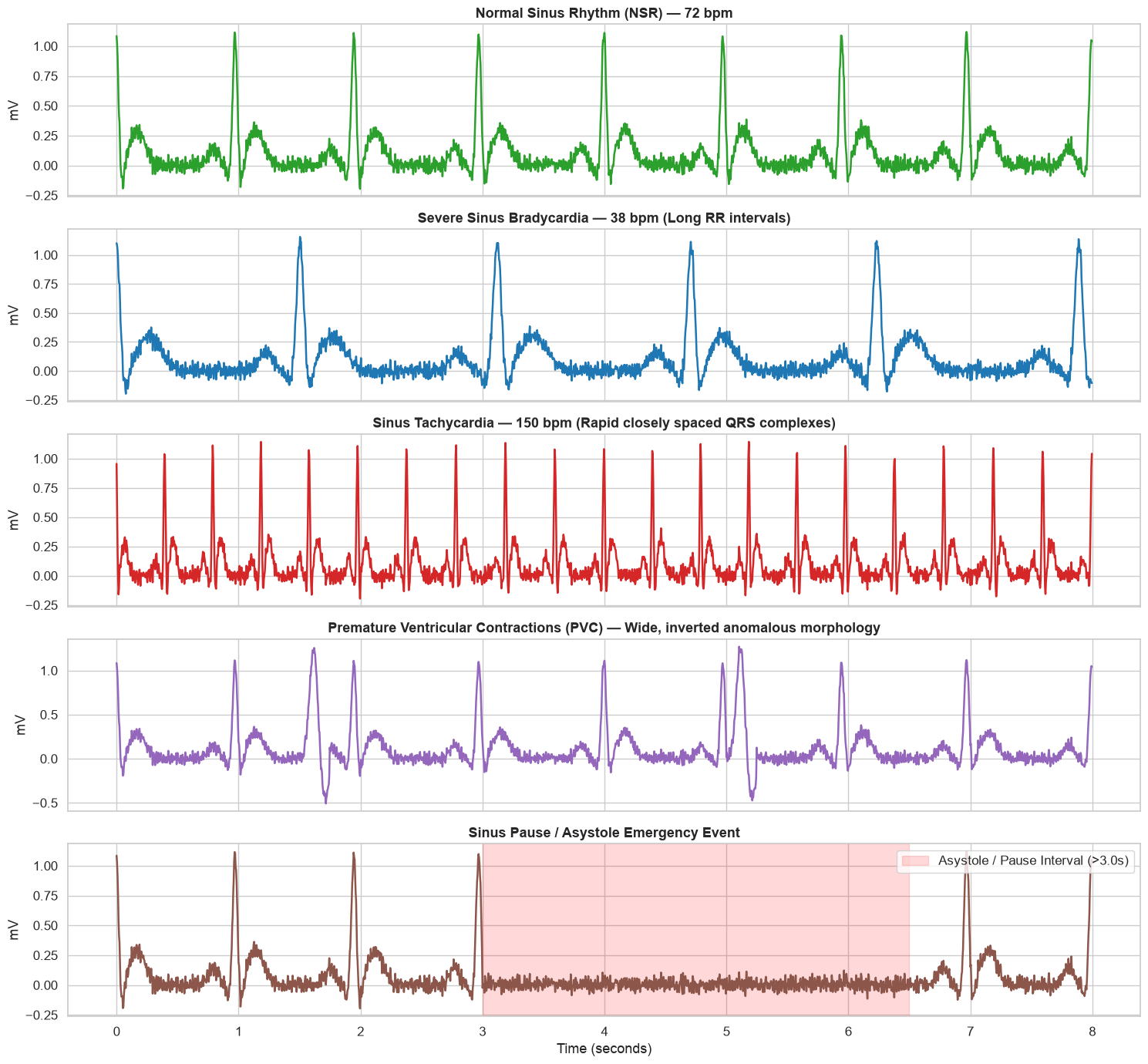
- Cardiac Arrhythmia Simulation: Inject Bradycardia, Tachycardia, PVCs, and Sinus Pause / Asystole.
- Clinical-Grade ECG Paper Plotting: 1:1 Physical Metric Scale (
display_mode="paper"— standard US Letter/A4 & thermal roll sizes) vs Responsive Screen Mode (display_mode="digital") with sparse tick label control.
1. Environment & Library Setup
import numpy as np
import pandas as pd
import matplotlib.pyplot as plt
import seaborn as sns

# Set modern visual styling
sns.set_theme(style="whitegrid", font_scale=1.1)
plt.rcParams["figure.figsize"] = (14, 6)
plt.rcParams["lines.linewidth"] = 1.8

# Import core SDK components, universal loaders & visualization
from ecg_sdk import (
    ECGSignal,
    load_ecg,
    load_mitbih_record,
    load_csv_record,
    save_to_csv,
    list_physionet_databases,
    list_mitbih_records,
    generate_synthetic_ecg,
    plot_clinical_ecg,
    plot_12lead_clinical,
)

print("✓ ecg_sdk universal loaders and visualization modules successfully imported!")
✓ ecg_sdk universal loaders and visualization modules successfully imported!
2. Exploring Supported PhysioNet Benchmark Databases
The SDK includes a built-in registry of clinical and benchmark databases across PhysioNet.
# View available PhysioNet benchmark databases
dbs = list_physionet_databases()
print("Supported Benchmark Databases:")
for db_id, info in dbs.items():
    print(f"  • {db_id:<10}: {info['name']} (Nominal fs={info.get('nominal_fs', 'N/A')} Hz)")

records = list_mitbih_records()
print(f"\nTotal MIT-BIH Standard Benchmark Records: {len(records)}")
print(f"Sample Record IDs: {records[:12]}...")
Supported Benchmark Databases:
  • mitdb     : MIT-BIH Arrhythmia Database (Nominal fs=360.0 Hz)
  • incartdb  : St. Petersburg INCART 12-lead Arrhythmia Database (Nominal fs=257.0 Hz)
  • ptb-xl    : PTB-XL 12-Lead Diagnostic ECG Database (Nominal fs=500.0 Hz)
  • nstdb     : MIT-BIH Noise Stress Test Database (Nominal fs=360.0 Hz)
  • afdb      : MIT-BIH Atrial Fibrillation Database (Nominal fs=250.0 Hz)
  • cudb      : Creighton University Ventricular Tachyarrhythmia Database (Nominal fs=250.0 Hz)
  • svdb      : MIT-BIH Supraventricular Arrhythmia Database (Nominal fs=128.0 Hz)
  • edb       : European ST-T Database (Nominal fs=250.0 Hz)
  • ludb      : Lobachevsky University Electrocardiography Database (Nominal fs=500.0 Hz)
  • fantasia  : Fantasia Database (Healthy Aging) (Nominal fs=250.0 Hz)

Total MIT-BIH Standard Benchmark Records: 48
Sample Record IDs: ['100', '101', '102', '103', '104', '105', '106', '107', '108', '109', '111', '112']...
3. Ingesting Benchmark Records in Physical mV vs Z-Score Normalization (load_ecg)
- Physical mV Scale (
normalize=None): Preserves actual voltages (typically -0.6 mV to +1.8 mV), ideal for 1:1 physical paper display. - Z-Score Normalization (
normalize="zscore"): Transforms the signal to zero mean and unit variance (std=1), required by neural network inputs.
# 1. Ingest MIT-BIH Record 101 (Textbook Sinus Rhythm in Physical mV, standardized to 250 Hz)
mit_101 = load_ecg(
    "physionet:mitdb/101",
    start_time=0.0,
    duration=10.0,
    target_fs=250.0,      # Standardize sampling frequency to 250 Hz
    normalize=None,       # Keep physical millivolts
    load_annotations=True,
)

print("✓ Standardized MIT-BIH Record 101 (Physical mV):")
print(mit_101)
print(f"Physical Voltage Range (MLII): [{np.min(mit_101.get_lead('MLII')):.3f} mV, {np.max(mit_101.get_lead('MLII')):.3f} mV]")

ann_101 = mit_101.metadata.get("annotations", {})
print(f"Proportionally Scaled R-Peaks: {len(ann_101.get('r_peaks', []))} beats")
print(f"R-Peak Sample Indices:         {ann_101.get('r_peaks', [])[:5]}")
✓ Standardized MIT-BIH Record 101 (Physical mV):
ECGSignal(record='101', leads=['MLII', 'V1'], fs=250.0Hz, duration=10.00s, shape=(2500, 2))
Physical Voltage Range (MLII): [-0.587 mV, 1.405 mV]
Proportionally Scaled R-Peaks: 12 beats
R-Peak Sample Indices:         [  5  58 275 494 717]
# 2. Stream St. Petersburg INCART 12-lead Record (257 Hz -> standardized to 250 Hz in physical mV)
incart_std = load_ecg(
    "I01",
    database="incartdb",
    start_time=0.0,
    duration=5.0,
    target_fs=250.0,
)

print("✓ Standardized INCART 12-Lead Record:")
print(incart_std)
print(f"Number of Leads: {incart_std.n_leads} ({incart_std.lead_names})")
✓ Standardized INCART 12-Lead Record:
ECGSignal(record='I01', leads=['I', 'II', 'III', 'aVR', 'aVL', 'aVF', 'V1', 'V2', 'V3', 'V4', 'V5', 'V6'], fs=250.0Hz, duration=5.00s, shape=(1250, 12))
Number of Leads: 12 (['I', 'II', 'III', 'aVR', 'aVL', 'aVF', 'V1', 'V2', 'V3', 'V4', 'V5', 'V6'])
4. Clinical Millimeter Paper Plotting (1:1 Physical Paper vs Digital Modes & Sparse Ticks)
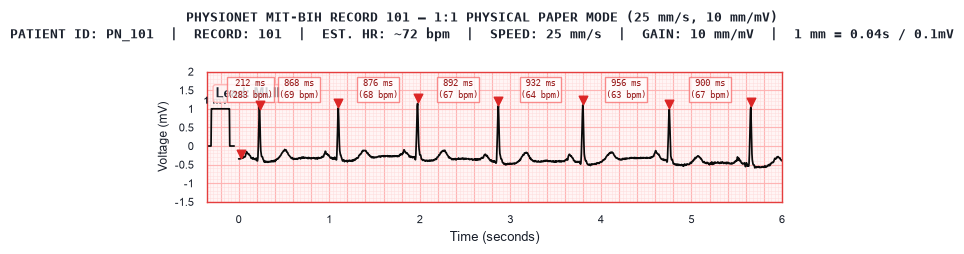
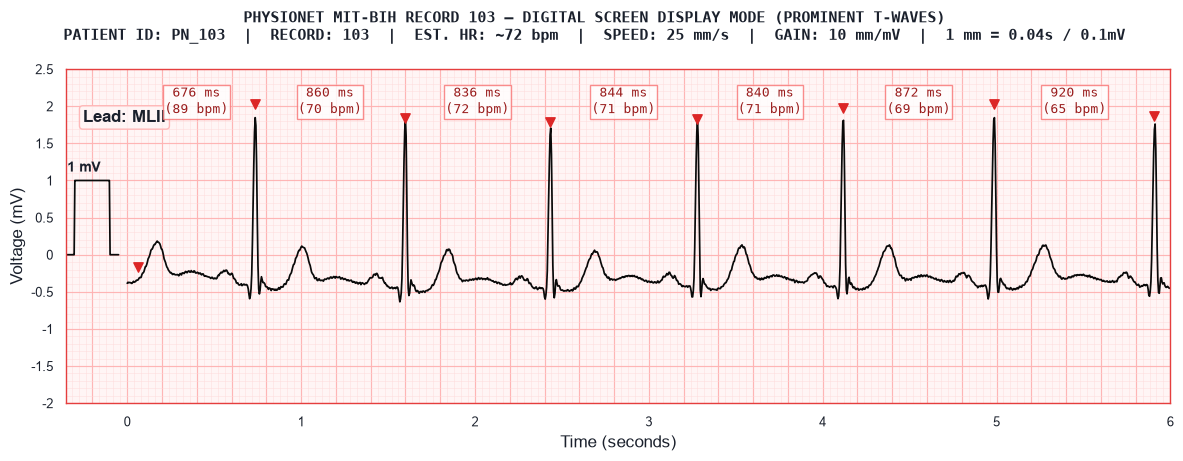
display_mode="paper"(Default): Exact 1:1 metric scale (25 mm/s, 10 mm/mV) matching physical medical thermal rolls (50 mm channel width).sparse_ticks=True: Unclutters the axis with clean labels (e.g. every 1.0 s and 0.5 mV) while preserving the complete 100% millimeter grid.
# 1. Plot MIT-BIH 101 on 1:1 Physical ECG Paper with Sparse Ticks
fig, ax = mit_101.plot_clinical(
    lead="MLII",
    duration=6.0,
    display_mode="paper",
    sparse_ticks=True,
    time_tick_step=1.0,      # Labels at 0, 1, 2, 3, 4, 5, 6 seconds
    voltage_tick_step=0.5,   # Labels at -0.5, 0.0, 0.5, 1.0, 1.5 mV
    grid_style="clinical_pink",
    r_peaks=ann_101.get("r_peaks"),
    show_calibration_pulse=True,
    title="PHYSIONET MIT-BIH RECORD 101 — 1:1 PHYSICAL PAPER MODE (25 mm/s, 10 mm/mV)",
)
plt.show()
# 2. Plot MIT-BIH 103 (Prominent P, QRS, T waves) in Digital Screen Mode
mit_103 = load_ecg("physionet:mitdb/103", duration=6.0, target_fs=250.0, load_annotations=True)
ann_103 = mit_103.metadata.get("annotations", {})

fig_dig, ax_dig = mit_103.plot_clinical(
    lead="MLII",
    duration=6.0,
    display_mode="digital",
    sparse_ticks=True,
    time_tick_step=1.0,
    voltage_tick_step=0.5,
    grid_style="clinical_pink",
    r_peaks=ann_103.get("r_peaks"),
    show_calibration_pulse=True,
    title="PHYSIONET MIT-BIH RECORD 103 — DIGITAL SCREEN DISPLAY MODE (PROMINENT T-WAVES)",
)
plt.show()
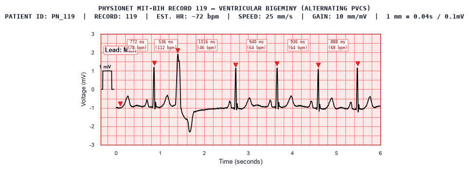
# 3. Ingest MIT-BIH Record 119 (Ventricular Bigeminy / Frequent PVCs) on Clinical Red Paper
mit_119 = load_ecg(
    "119",
    database="mitdb",
    start_time=0.0,
    duration=6.0,
    target_fs=250.0,
    load_annotations=True,
)
ann_119 = mit_119.metadata.get("annotations", {})

fig, ax = mit_119.plot_clinical(
    lead="MLII",
    duration=6.0,
    display_mode="paper",
    sparse_ticks=True,
    time_tick_step=1.0,
    voltage_tick_step=1.0,
    grid_style="clinical_red",
    r_peaks=ann_119.get("r_peaks"),
    show_calibration_pulse=True,
    title="PHYSIONET MIT-BIH RECORD 119 — VENTRICULAR BIGEMINY (ALTERNATING PVCS)",
)
plt.show()
5. Exploring ECGSignal Transformations (Slicing, Resampling, Normalization, DataFrames)
# Statistical summary of the real standardized clinical record
import pprint
pprint.pprint(mit_101.summary())
{'duration_sec': 10.0,
 'leads': {'MLII': {'max': 1.4054778388413307,
                    'mean': -0.31201111111111113,
                    'min': -0.5873070562653526,
                    'peak_to_peak': 1.9927848951066833,
                    'std': 0.1991377319242747},
           'V1': {'max': -0.056206449218917896,
                  'mean': -0.14991111111111108,
                  'min': -0.40859738192043565,
                  'peak_to_peak': 0.3523909327015178,
                  'std': 0.04272543866254888}},
 'n_leads': 2,
 'n_samples': 2500,
 'patient_id': 'PN_101',
 'record_name': '101',
 'sampling_rate': 250.0,
 'units': 'mV'}
| time_sec | MLII | V1 | |
|---|---|---|---|
| 0 | 0.000 | -0.345565 | -0.149839 |
| 1 | 0.004 | -0.344463 | -0.163473 |
| 2 | 0.008 | -0.345456 | -0.157958 |
| 3 | 0.012 | -0.344521 | -0.161417 |
| 4 | 0.016 | -0.345759 | -0.159056 |
| 5 | 0.020 | -0.341805 | -0.159222 |
| 6 | 0.024 | -0.322545 | -0.144194 |
| 7 | 0.028 | -0.320184 | -0.170237 |
| 8 | 0.032 | -0.328091 | -0.177091 |
| 9 | 0.036 | -0.326013 | -0.152641 |
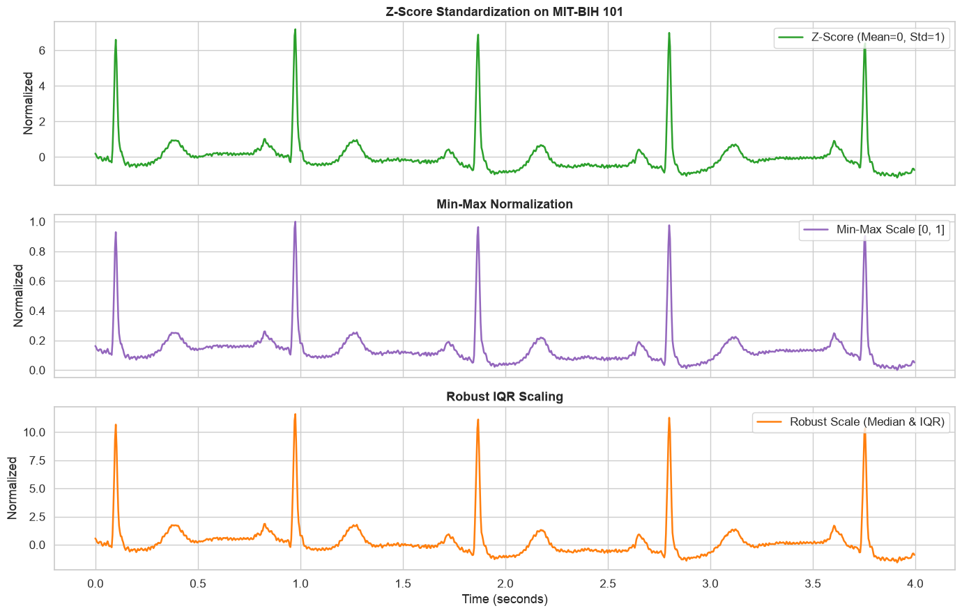
# Slice a 4-second zoom window
mit_zoom = mit_101.slice(start_time=1.0, end_time=5.0)

# Apply 3 normalization strategies
norm_z = mit_zoom.normalize(method="zscore")
norm_minmax = mit_zoom.normalize(method="minmax")
norm_robust = mit_zoom.normalize(method="robust")

fig, axes = plt.subplots(3, 1, figsize=(14, 9), sharex=True)

axes[0].plot(norm_z.time_vector, norm_z.get_lead("MLII"), color="#2ca02c", label="Z-Score (Mean=0, Std=1)")
axes[0].set_ylabel("Normalized")
axes[0].set_title("Z-Score Standardization on MIT-BIH 101", fontweight="bold")
axes[0].legend(loc="upper right")

axes[1].plot(norm_minmax.time_vector, norm_minmax.get_lead("MLII"), color="#9467bd", label="Min-Max Scale [0, 1]")
axes[1].set_ylabel("Normalized")
axes[1].set_title("Min-Max Normalization", fontweight="bold")
axes[1].legend(loc="upper right")

axes[2].plot(norm_robust.time_vector, norm_robust.get_lead("MLII"), color="#ff7f0e", label="Robust Scale (Median & IQR)")
axes[2].set_xlabel("Time (seconds)")
axes[2].set_ylabel("Normalized")
axes[2].set_title("Robust IQR Scaling", fontweight="bold")
axes[2].legend(loc="upper right")

plt.tight_layout()
plt.show()
6. McSharry Dynamical Synthetic ECG Generator (12-Lead Vectorcardiography)
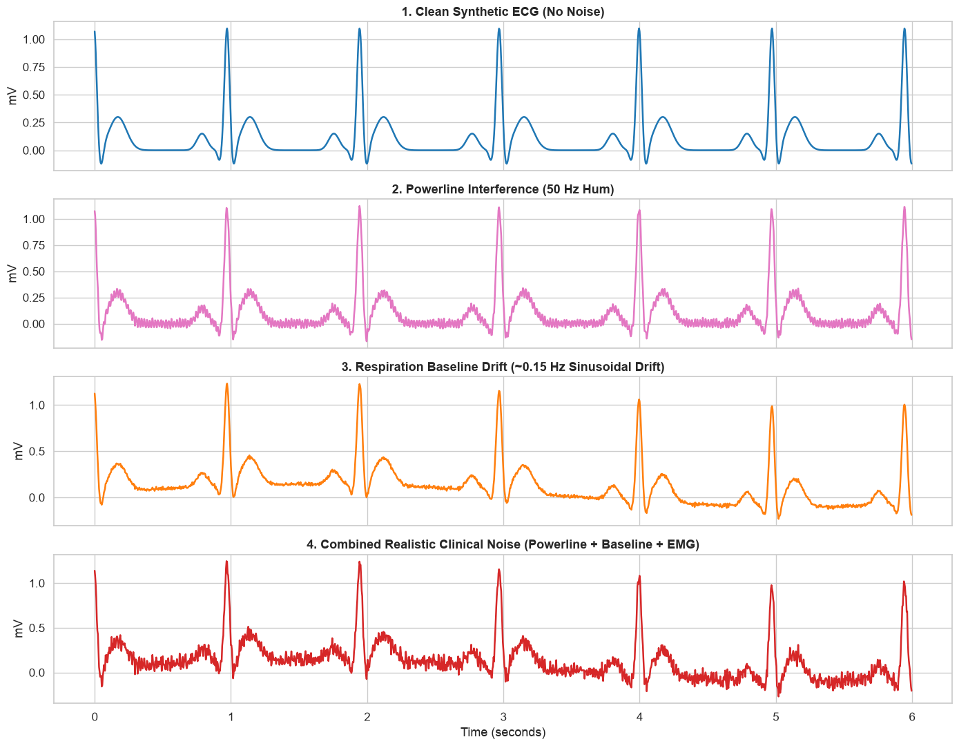
The generator implements the seminal McSharry (2003) and Sameni (2007) dynamical equations with authentic 12-lead parameters (Einthoven limb leads, inverted aVR, and precordial R-wave progression V1 -> V6).
# 1. Clean Reference
clean_sig = generate_synthetic_ecg(duration=6.0, sampling_rate=250.0, noise_level=0.0, powerline_hz=None, baseline_wander=False)

# 2. With 50 Hz Powerline Noise
powerline_sig = generate_synthetic_ecg(duration=6.0, sampling_rate=250.0, noise_level=0.01, powerline_hz=50.0, baseline_wander=False)

# 3. With Respiration Baseline Wander
wander_sig = generate_synthetic_ecg(duration=6.0, sampling_rate=250.0, noise_level=0.01, powerline_hz=None, baseline_wander=True)

# 4. Combined Realistic Clinical Artifacts
realistic_sig = generate_synthetic_ecg(duration=6.0, sampling_rate=250.0, noise_level=0.04, powerline_hz=50.0, baseline_wander=True)

fig, axes = plt.subplots(4, 1, figsize=(14, 11), sharex=True)

axes[0].plot(clean_sig.time_vector, clean_sig.get_lead(0), color="#1f77b4")
axes[0].set_title("1. Clean Synthetic ECG (No Noise)", fontweight="bold")
axes[0].set_ylabel("mV")

axes[1].plot(powerline_sig.time_vector, powerline_sig.get_lead(0), color="#e377c2")
axes[1].set_title("2. Powerline Interference (50 Hz Hum)", fontweight="bold")
axes[1].set_ylabel("mV")

axes[2].plot(wander_sig.time_vector, wander_sig.get_lead(0), color="#ff7f0e")
axes[2].set_title("3. Respiration Baseline Drift (~0.15 Hz Sinusoidal Drift)", fontweight="bold")
axes[2].set_ylabel("mV")

axes[3].plot(realistic_sig.time_vector, realistic_sig.get_lead(0), color="#d62728")
axes[3].set_title("4. Combined Realistic Clinical Noise (Powerline + Baseline + EMG)", fontweight="bold")
axes[3].set_xlabel("Time (seconds)")
axes[3].set_ylabel("mV")

plt.tight_layout()
plt.show()
7. Cardiac Arrhythmia Gallery
duration = 8.0
fs = 250.0

sig_nsr = generate_synthetic_ecg(duration=duration, sampling_rate=fs, anomaly="normal", baseline_wander=False)
sig_brady = generate_synthetic_ecg(duration=duration, sampling_rate=fs, anomaly="bradycardia", baseline_wander=False)
sig_tachy = generate_synthetic_ecg(duration=duration, sampling_rate=fs, anomaly="tachycardia", baseline_wander=False)
sig_pvc = generate_synthetic_ecg(duration=duration, sampling_rate=fs, anomaly="pvc", baseline_wander=False)
sig_pause = generate_synthetic_ecg(duration=duration, sampling_rate=fs, anomaly="pause", baseline_wander=False)

fig, axes = plt.subplots(5, 1, figsize=(15, 14), sharex=True)

axes[0].plot(sig_nsr.time_vector, sig_nsr.get_lead(0), color="#2ca02c")
axes[0].set_title("Normal Sinus Rhythm (NSR) — 72 bpm", fontweight="bold")
axes[0].set_ylabel("mV")

axes[1].plot(sig_brady.time_vector, sig_brady.get_lead(0), color="#1f77b4")
axes[1].set_title("Severe Sinus Bradycardia — 38 bpm (Long RR intervals)", fontweight="bold")
axes[1].set_ylabel("mV")

axes[2].plot(sig_tachy.time_vector, sig_tachy.get_lead(0), color="#d62728")
axes[2].set_title("Sinus Tachycardia — 150 bpm (Rapid closely spaced QRS complexes)", fontweight="bold")
axes[2].set_ylabel("mV")

axes[3].plot(sig_pvc.time_vector, sig_pvc.get_lead(0), color="#9467bd")
axes[3].set_title("Premature Ventricular Contractions (PVC) — Wide, inverted anomalous morphology", fontweight="bold")
axes[3].set_ylabel("mV")

axes[4].plot(sig_pause.time_vector, sig_pause.get_lead(0), color="#8c564b")
axes[4].axvspan(3.0, 6.5, color="red", alpha=0.15, label="Asystole / Pause Interval (>3.0s)")
axes[4].set_title("Sinus Pause / Asystole Emergency Event", fontweight="bold")
axes[4].set_xlabel("Time (seconds)")
axes[4].set_ylabel("mV")
axes[4].legend(loc="upper right")

plt.tight_layout()
plt.show()
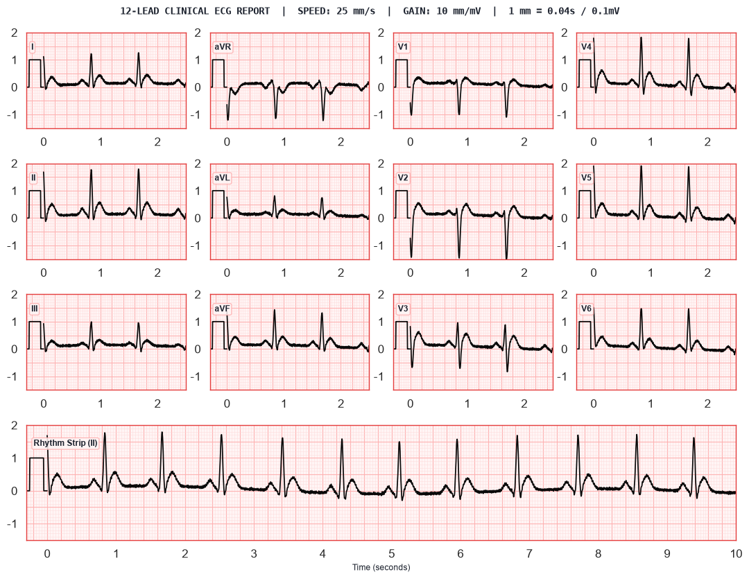
8. Standard 12-Lead Diagnostic Clinical Report Layout (3x4 + 1 Rhythm Strip)
Standard hospital printout on US Letter Landscape (11.0" x 8.5") or ISO A4 Landscape (11.69" x 8.27").
# Generate 12-lead synthetic recording with authentic canonical parameters
canonical_12_leads = ["I", "II", "III", "aVR", "aVL", "aVF", "V1", "V2", "V3", "V4", "V5", "V6"]
ecg_12lead = generate_synthetic_ecg(
    duration=10.0,
    sampling_rate=250.0,
    heart_rate=70.0,
    noise_level=0.01,
    lead_names=canonical_12_leads,
    random_seed=42,
)
ecg_12lead.record_name = "PTB_12LEAD_BENCHMARK"
ecg_12lead.patient_id = "HOSPITAL_PATIENT_1029"

# Plot standard 3x4 + rhythm layout in 1:1 Physical Paper Mode (US Letter Landscape 11.0" x 8.5") with sparse ticks
fig12, axes12 = plot_12lead_clinical(
    signal=ecg_12lead,
    duration=2.5,
    display_mode="paper",
    paper_size="letter",
    sparse_ticks=True,
    time_tick_step=1.0,
    voltage_tick_step=1.0,
    grid_style="clinical_pink",
    voltage_range=(-1.5, 2.0),
    rhythm_lead="II",
)
plt.show()
9. CSV Round-Trip Serialization
import os
import tempfile

# Create temporary CSV file
with tempfile.NamedTemporaryFile(suffix=".csv", delete=False) as tmp:
    tmp_path = tmp.name

try:
    # Save synthetic signal
    save_to_csv(sig_pvc, tmp_path)
    print(f"✓ Saved ECGSignal to: {tmp_path}")

    # Load back
    loaded_ecg = load_csv_record(tmp_path, sampling_rate=250.0)
    print(f"✓ Loaded back: {loaded_ecg}")

    # Verify numerical match
    np.testing.assert_allclose(sig_pvc.data, loaded_ecg.data, rtol=1e-5, atol=1e-5)
    print("✓ Numerical verification passed (Data is identical)!")
finally:
    if os.path.exists(tmp_path):
        os.remove(tmp_path)
✓ Saved ECGSignal to: /var/folders/1h/9mghv8bj2_7g5bvgd79rb0bw0000gn/T/tmpaf9anvks.csv
✓ Loaded back: ECGSignal(record='tmpaf9anvks', leads=['Lead_I', 'Lead_II'], fs=250.0Hz, duration=8.00s, shape=(2000, 2))
✓ Numerical verification passed (Data is identical)!