Tutorial 02: Digital Filtering, Baseline Wander Removal & Signal Quality Index (SQI)¶

In clinical electrocardiography and edge telemetry, biopotential recordings are routinely corrupted by physiological and environmental noise sources: 1. Powerline Interference (50 Hz / 60 Hz): AC mains hum coupling into high-impedance skin-electrode interfaces. 2. Respiratory Baseline Wander (0.05–0.5 Hz): Patient breathing, perspiration, and thoracic impedance shifts. 3. Electromyographic (EMG) Noise (>40 Hz): Somatic muscle tremors and motion artifacts. 4. Electrode Motion / Detachment: High-amplitude transient baseline jumps or flatlines.

This tutorial demonstrates the signal conditioning and quality assessment capabilities of the AI ECG SDK (ecg_sdk).

import numpy as np
import matplotlib.pyplot as plt
from scipy import signal as scipy_signal

import ecg_sdk
from ecg_sdk.core.signal import ECGSignal
from ecg_sdk.core.generator import generate_synthetic_ecg
from ecg_sdk.core.loaders import load_mitbih_record
from ecg_sdk.preprocessing.filters import (
    butter_bandpass_filter,
    iir_notch_filter,
    filter_ecg,
)
from ecg_sdk.preprocessing.baseline import (
    cascaded_median_baseline_wander,
    remove_baseline_wander,
)
from ecg_sdk.preprocessing.quality import (
    assess_signal_quality,
    calculate_psqi,
    calculate_ksqi,
)

print(f"ai-ecg-sdk version: {ecg_sdk.__version__}")

ai-ecg-sdk version: 0.1.0

1. Digital Filtering: Butterworth Bandpass & IIR Notch Filter¶

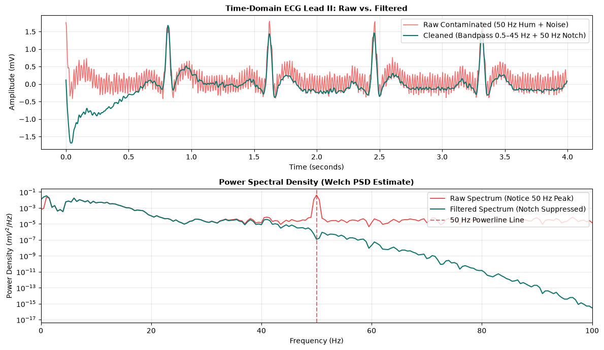
We synthesize a multi-lead ECG contaminated with 50 Hz powerline hum (\(0.25\text{ mV}\)) and EMG tremor noise (\(0.05\text{ mV}\)).

# 1. Generate noisy ECG (50 Hz hum + high-frequency noise)
raw_noisy_ecg = generate_synthetic_ecg(
    duration=6.0,
    sampling_rate=250.0,
    heart_rate=72.0,
    leads=["I", "II", "V1"],
    noise_level=0.06,
    powerline_hz=50.0,
    powerline_noise=0.25,
    baseline_wander=False,
    random_seed=42,
)

# 2. Apply zero-phase Butterworth bandpass (0.5-45 Hz) + 50 Hz IIR Notch filter
filtered_ecg = raw_noisy_ecg.filter(lowcut=0.5, highcut=45.0, notch_freq=50.0, notch_q=30.0)

print("Raw Signal:", raw_noisy_ecg)
print("Filtered Signal:", filtered_ecg)
print("Filter Metadata:", filtered_ecg.metadata.get("preprocessing_filters"))

Raw Signal: ECGSignal(record='SYNTH_NORMAL', leads=['I', 'II', 'V1'], fs=250.0Hz, duration=6.00s, shape=(1500, 3))
Filtered Signal: ECGSignal(record='SYNTH_NORMAL', leads=['I', 'II', 'V1'], fs=250.0Hz, duration=6.00s, shape=(1500, 3))
Filter Metadata: {'bandpass': (0.5, 45.0), 'notch_freq': 50.0, 'order': 4}

1.1 Visualizing Power Spectral Density (PSD) Before vs. After Filtering¶

Using Welch's periodogram, we observe the exact notch cancellation of the 50 Hz spike and high-frequency roll-off above 45 Hz.

fig, (ax_time, ax_psd) = plt.subplots(2, 1, figsize=(12, 7))

t = raw_noisy_ecg.time_vector[:1000]
raw_lead2 = raw_noisy_ecg.get_lead("II")[:1000]
filt_lead2 = filtered_ecg.get_lead("II")[:1000]

# Time domain comparison
ax_time.plot(t, raw_lead2, label="Raw Contaminated (50 Hz Hum + Noise)", color="#ef4444", alpha=0.75, lw=1.2)
ax_time.plot(t, filt_lead2, label="Cleaned (Bandpass 0.5–45 Hz + 50 Hz Notch)", color="#0f766e", lw=1.5)
ax_time.set_title("Time-Domain ECG Lead II: Raw vs. Filtered", fontweight="bold", fontsize=11)
ax_time.set_xlabel("Time (seconds)")
ax_time.set_ylabel("Amplitude (mV)")
ax_time.grid(True, alpha=0.3)
ax_time.legend(loc="upper right", frameon=True)

# Frequency domain PSD comparison
f_raw, psd_raw = scipy_signal.welch(raw_noisy_ecg.get_lead("II"), fs=250.0, nperseg=500)
f_filt, psd_filt = scipy_signal.welch(filtered_ecg.get_lead("II"), fs=250.0, nperseg=500)

ax_psd.semilogy(f_raw, psd_raw, label="Raw Spectrum (Notice 50 Hz Peak)", color="#ef4444", lw=1.3)
ax_psd.semilogy(f_filt, psd_filt, label="Filtered Spectrum (Notch Suppressed)", color="#0f766e", lw=1.5)
ax_psd.axvline(50.0, color="#b91c1c", linestyle="--", alpha=0.6, label="50 Hz Powerline Line")
ax_psd.set_title("Power Spectral Density (Welch PSD Estimate)", fontweight="bold", fontsize=11)
ax_psd.set_xlabel("Frequency (Hz)")
ax_psd.set_ylabel("Power Density ($mV^2 / Hz$)")
ax_psd.set_xlim(0, 100)
ax_psd.grid(True, which="both", alpha=0.3)
ax_psd.legend(loc="upper right", frameon=True)

plt.tight_layout()
plt.show()

png

2. Two-Stage Cascaded Median Baseline Wander Removal¶

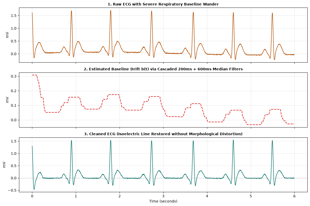
Baseline wander caused by respiration (\(\sim 0.15\text{--}0.3\text{ Hz}\)) introduces low-frequency voltage oscillations. To avoid distorting ST segments or T-wave amplitudes (which linear highpass filters can distort), we implement the two-stage cascaded median filter (de Chazal et al., 2004): - Stage 1 (200 ms): Removes narrow P-waves and QRS complexes. - Stage 2 (600 ms): Removes wide T-waves, isolating the slow baseline drift \(\mathbf{b}(t)\). - Output: \(\tilde{\mathbf{x}}(t) = \mathbf{x}(t) - \mathbf{b}(t)\).

# Generate ECG with severe respiratory baseline wander
drift_ecg = generate_synthetic_ecg(
    duration=6.0,
    sampling_rate=250.0,
    heart_rate=65.0,
    leads=["II"],
    noise_level=0.01,
    powerline_hz=None,
    baseline_wander=0.45,  # Heavy respiratory drift
    random_seed=123,
)

# Extract and remove baseline drift
detrended_ecg, estimated_baseline = drift_ecg.remove_baseline(
    method="cascaded_median",
    window1_ms=200.0,
    window2_ms=600.0,
    return_baseline=True,
)

fig, axes = plt.subplots(3, 1, figsize=(12, 8), sharex=True)
t = drift_ecg.time_vector

axes[0].plot(t, drift_ecg.get_lead(0), color="#b45309", lw=1.3)
axes[0].set_title("1. Raw ECG with Severe Respiratory Baseline Wander", fontweight="bold", fontsize=10)
axes[0].set_ylabel("mV")
axes[0].grid(True, alpha=0.3)

axes[1].plot(t, estimated_baseline, color="#dc2626", lw=1.6, linestyle="--")
axes[1].set_title("2. Estimated Baseline Drift b(t) via Cascaded 200ms + 600ms Median Filters", fontweight="bold", fontsize=10)
axes[1].set_ylabel("mV")
axes[1].grid(True, alpha=0.3)

axes[2].plot(t, detrended_ecg.get_lead(0), color="#0f766e", lw=1.3)
axes[2].axhline(0, color="gray", linestyle=":", alpha=0.5)
axes[2].set_title("3. Cleaned ECG (Isoelectric Line Restored without Morphological Distortion)", fontweight="bold", fontsize=10)
axes[2].set_xlabel("Time (seconds)")
axes[2].set_ylabel("mV")
axes[2].grid(True, alpha=0.3)

plt.tight_layout()
plt.show()

png

3. Real Clinical ECG Preprocessing: PhysioNet MIT-BIH Arrhythmia Database¶

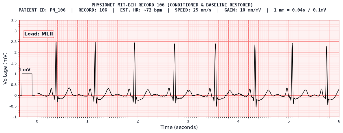
Let's test the conditioning pipeline on real patient recordings from PhysioNet MIT-BIH (mitdb/101 and mitdb/106).

# Load real MIT-BIH record 106 (frequent ventricular ectopy & baseline variation)
mit_106_raw = load_mitbih_record("106", start_time=20.0, duration=8.0)

# Apply unified conditioning: Bandpass (0.5-45 Hz) + Notch (60 Hz US powerline) + Cascaded Median
mit_106_clean = mit_106_raw.filter(lowcut=0.5, highcut=45.0, notch_freq=60.0).remove_baseline()

# Render clinical paper plot of cleaned recording
fig, _ = mit_106_clean.plot_clinical(
    lead="MLII",
    duration=6.0,
    display_mode="digital",
    grid_style="clinical_red",
    title="PHYSIONET MIT-BIH RECORD 106 (CONDITIONED & BASELINE RESTORED)",
)
plt.show()

findfont: Failed to find font weight medium, now using 400.


findfont: Failed to find font weight medium, now using 400.

png

4. Multi-Metric Signal Quality Index (SQI) Engine¶

The SDK includes a multi-dimensional Signal Quality Index (SQI) framework based on Clifford et al. (2012) and Orphanidou et al. (2015): - \(p\text{SQI}\) (Power Spectrum Ratio): Energy concentration in the diagnostic QRS band (\(5\text{--}15\text{ Hz}\)) vs total physiological band (\(5\text{--}40\text{ Hz}\)). - \(k\text{SQI}\) (Kurtosis): High values (\(>5.0\)) indicate impulsive, sharp QRS complexes; Gaussian noise yields \(\kappa \approx 3.0\). - \(s\text{SQI}\) (Skewness): Degree of biopotential distribution asymmetry. - \(\text{basSQI}\) (Baseline Drift Index): Ratio of energy \(<0.5\text{ Hz}\) to total ECG energy. - \(\text{hfSQI}\) (High-Frequency Noise Index): Ratio of power \(>45\text{ Hz}\) to total ECG energy. - Composite Score: Normalized index \(\in [0, 1]\) grading signals into excellent, acceptable, or unusable.

# Compare SQI across 3 signal conditions:
# 1. Clean synthetic signal
clean_sig = generate_synthetic_ecg(duration=10.0, sampling_rate=250.0, noise_level=0.01, baseline_wander=False)
sqi_clean = clean_sig.assess_quality()

# 2. Noisy signal with heavy drift and hum
noisy_sig = generate_synthetic_ecg(duration=10.0, sampling_rate=250.0, noise_level=0.15, powerline_noise=0.4, baseline_wander=0.6)
sqi_noisy = noisy_sig.assess_quality()

# 3. Disconnected / flatline recording
flatline_sig = ECGSignal(data=np.zeros((2500, 2)), sampling_rate=250.0, lead_names=["I", "II"])
sqi_flatline = flatline_sig.assess_quality()

print(sqi_clean.summary())
print("\n" + sqi_noisy.summary())
print("\n" + sqi_flatline.summary())

====================================================================
SIGNAL QUALITY ASSESSMENT REPORT (SQI)
====================================================================
Overall Composite SQI : 0.997 / 1.000
Overall Quality Grade : EXCELLENT
Acceptable for AI/ML  : YES [✓]
--------------------------------------------------------------------
Lead       pSQI     kSQI     basSQI    hfSQI    Score    Grade
--------------------------------------------------------------------
Lead_I     0.984    12.68    0.000     0.013    0.996    excellent
Lead_II    0.985    13.46    0.000     0.006    0.998    excellent
====================================================================

====================================================================
SIGNAL QUALITY ASSESSMENT REPORT (SQI)
====================================================================
Overall Composite SQI : 0.655 / 1.000
Overall Quality Grade : ACCEPTABLE
Acceptable for AI/ML  : YES [✓]
--------------------------------------------------------------------
Lead       pSQI     kSQI     basSQI    hfSQI    Score    Grade
--------------------------------------------------------------------
Lead_I     0.866    3.27     0.000     1.688    0.596    unusable
Lead_II    0.932    5.25     0.000     0.821    0.715    acceptable
====================================================================

====================================================================
SIGNAL QUALITY ASSESSMENT REPORT (SQI)
====================================================================
Overall Composite SQI : 0.000 / 1.000
Overall Quality Grade : UNUSABLE
Acceptable for AI/ML  : NO [✗]
--------------------------------------------------------------------
Lead       pSQI     kSQI     basSQI    hfSQI    Score    Grade
--------------------------------------------------------------------
I          0.000    0.00     1.000     1.000    0.000    unusable
II         0.000    0.00     1.000     1.000    0.000    unusable
====================================================================

4.1 Tabular Quality Benchmark Table¶

import pandas as pd

records_to_test = {
    "Clean Synthetic (Lead II)": clean_sig.get_lead("II"),
    "Noisy Contaminated (Lead II)": noisy_sig.get_lead("II"),
    "Conditioned Noisy (Lead II)": noisy_sig.filter().remove_baseline().get_lead("II"),
    "Flatline Disconnected": np.zeros(2500),
    "Real MIT-BIH 101 (MLII)": load_mitbih_record("101", duration=10.0).get_lead(0),
}

rows = []
for name, data_arr in records_to_test.items():
    report = assess_signal_quality(data_arr, fs=250.0, lead_names=["Lead"])
    lead_q = report.lead_metrics["Lead"]
    rows.append({
        "Signal Description": name,
        "pSQI (QRS Energy)": f"{lead_q.psqi:.3f}",
        "kSQI (Kurtosis)": f"{lead_q.ksqi:.2f}",
        "basSQI (Drift Ratio)": f"{lead_q.bas_sqi:.3f}",
        "hfSQI (Noise Ratio)": f"{lead_q.hf_sqi:.3f}",
        "Composite SQI": f"{lead_q.composite_sqi:.3f}",
        "Quality Grade": lead_q.grade.upper(),
        "Acceptable for AI": "YES [✓]" if lead_q.is_acceptable else "NO [✗]",
    })

df_sqi = pd.DataFrame(rows)
df_sqi

	Signal Description	pSQI (QRS Energy)	kSQI (Kurtosis)	basSQI (Drift Ratio)	hfSQI (Noise Ratio)	Composite SQI	Quality Grade	Acceptable for AI
0	Clean Synthetic (Lead II)	0.985	13.46	0.000	0.006	0.998	EXCELLENT	YES [✓]
1	Noisy Contaminated (Lead II)	0.932	5.25	0.000	0.821	0.715	ACCEPTABLE	YES [✓]
2	Conditioned Noisy (Lead II)	0.936	13.72	0.000	0.001	1.000	EXCELLENT	YES [✓]
3	Flatline Disconnected	0.000	0.00	1.000	1.000	0.000	UNUSABLE	NO [✗]
4	Real MIT-BIH 101 (MLII)	0.774	30.18	0.000	0.001	1.000	EXCELLENT	YES [✓]

Summary of Key Takeaways¶

Zero-Phase Digital Filtering (sig.filter()): Effectively removes 50/60 Hz powerline hum and high-frequency EMG tremor while maintaining precise temporal alignment of all fiducial points.
Cascaded Median Filtering (sig.remove_baseline()): Eliminates respiratory baseline wander without introducing artificial ST elevation or depression.
Multi-Metric SQI (sig.assess_quality()): Provides automated gating for clinical AI models, ensuring corrupted or disconnected leads are caught before inference.